Logarithm. Natural logarithm
The basic properties of the natural logarithm, graph, domain of definition, set of values, basic formulas, derivative, integral, power series expansion and representation of the function ln x using complex numbers are given.
Definition
Natural logarithm is the function y = ln x, the inverse of the exponential, x = e y, and is the logarithm to the base of the number e: ln x = log e x.
The natural logarithm is widely used in mathematics because its derivative has the simplest form: (ln x)′ = 1/ x.
Based definitions, the base of the natural logarithm is the number e:
e ≅ 2.718281828459045...;
.
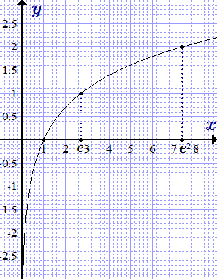
Graph of the function y = ln x.
Graph of natural logarithm (functions y = ln x) is obtained from the exponential graph mirror image relative to the straight line y = x.
The natural logarithm is defined for positive values of the variable x.
It increases monotonically in its domain of definition. 0 At x →
the limit of the natural logarithm is minus infinity (-∞).
As x → + ∞, the limit of the natural logarithm is plus infinity (+ ∞). For large x, the logarithm increases quite slowly. Any power function x a with a positive exponent a grows faster than the logarithm.
Properties of the natural logarithm
Domain of definition, set of values, extrema, increase, decrease
The natural logarithm is a monotonically increasing function, so it has no extrema. The main properties of the natural logarithm are presented in the table.
ln x values
ln 1 = 0
Basic formulas for natural logarithms
Formulas following from the definition of the inverse function:
The main property of logarithms and its consequences
Base replacement formula
Any logarithm can be expressed in terms of natural logarithms using the base substitution formula:
Proofs of these formulas are presented in the section "Logarithm".
Inverse function
The inverse of the natural logarithm is the exponent.
If , then
If, then.
Derivative ln x
.
Derivative of the natural logarithm:
.
Derivative of the natural logarithm of modulus x:
.
Derivative of nth order:
Deriving formulas > > >
Integral
.
The integral is calculated by integration by parts:
So,
Expressions using complex numbers
.
Consider the function of the complex variable z: Let's express the complex variable z via module r φ
:
.
and argument
.
Using the properties of the logarithm, we have:
.
Or
The argument φ is not uniquely defined. If you put
, where n is an integer,
Therefore, the natural logarithm, as a function of a complex variable, is not a single-valued function.
Power series expansion
When the expansion takes place:
References:
I.N. Bronstein, K.A. Semendyaev, Handbook of mathematics for engineers and college students, “Lan”, 2009.
often take a number e = 2,718281828 . Logarithms based on this base are called natural. When performing calculations with natural logarithms, it is common to operate with the sign ln, but not log; while the number 2,718281828 , defining the basis, are not indicated.
In other words, the formulation will look like: natural logarithm numbers X- this is an exponent to which a number must be raised e, To obtain x.
So, ln(7,389...)= 2, since e 2 =7,389... . Natural logarithm of the number itself e= 1 because e 1 =e, and the natural logarithm of unity equal to zero, because e 0 = 1.
The number itself e defines the limit of a monotonic bounded sequence
it is calculated that e = 2,7182818284... .
Quite often, in order to fix a number in memory, the digits of the required number are associated with some outstanding date. Speed of memorizing the first nine digits of a number e after the decimal point will increase if you notice that 1828 is the year of birth of Leo Tolstoy!
Today there are quite complete tables of natural logarithms.
Natural logarithm graph(functions y=ln x) is a consequence of the exponent graph being a mirror image of the straight line y = x and has the form:

The natural logarithm can be found for every positive real number a as the area under the curve y = 1/x from 1 before a.
The elementary nature of this formulation, which is consistent with many other formulas in which the natural logarithm is involved, was the reason for the formation of the name “natural”.
If you analyze natural logarithm, as a real function of a real variable, then it acts inverse function to an exponential function, which reduces to the identities:
e ln(a) =a (a>0)
ln(e a) =a
By analogy with all logarithms, the natural logarithm converts multiplication into addition, division into subtraction:
ln(xy) = ln(x) + ln(y)
ln(x/y)= lnx - lny
The logarithm can be found for every positive base that is not equal to one, not just for e, but logarithms for other bases differ from the natural logarithm only by a constant factor, and are usually defined in terms of the natural logarithm.
Having analyzed natural logarithm graph, we find that it exists for positive values of the variable x. It increases monotonically in its domain of definition.
At x → 0 the limit of the natural logarithm is minus infinity ( -∞ ).At x → +∞ the limit of the natural logarithm is plus infinity ( + ∞ ). At large x The logarithm increases quite slowly. Any power function xa with a positive exponent a increases faster than the logarithm. The natural logarithm is a monotonically increasing function, so it has no extrema.
Usage natural logarithms very rational when passing higher mathematics. Thus, using the logarithm is convenient for finding the answer to equations in which unknowns appear as exponents. The use of natural logarithms in calculations makes it possible to greatly simplify a large number of mathematical formulas. Logarithms to the base e are present in solving a significant number of physical problems and are naturally included in mathematical description individual chemical, biological and other processes. Thus, logarithms are used to calculate the decay constant for a known half-life, or to calculate the decay time in solving problems of radioactivity. They perform in leading role in many branches of mathematics and practical sciences, they are used in the field of finance to solve a large number of problems, including the calculation of compound interest.
The logarithm of a positive number b to base a (a>0, a is not equal to 1) is a number c such that a c = b: log a b = c ⇔ a c = b (a > 0, a ≠ 1, b > 0)
Note that the logarithm of a non-positive number is undefined. In addition, the base of the logarithm must be a positive number that is not equal to 1. For example, if we square -2, we get the number 4, but this does not mean that the base -2 logarithm of 4 is equal to 2.
Basic logarithmic identity
a log a b = b (a > 0, a ≠ 1) (2)It is important that the scope of definition of the right and left sides of this formula is different. Left side is defined only for b>0, a>0 and a ≠ 1. The right-hand side is defined for any b, and does not depend on a at all. Thus, the application of the basic logarithmic “identity” when solving equations and inequalities can lead to a change in the OD.
Two obvious consequences of the definition of logarithm
log a a = 1 (a > 0, a ≠ 1) (3)log a 1 = 0 (a > 0, a ≠ 1) (4)
Indeed, when raising the number a to the first power, we get the same number, and when raising it to the zero power, we get one.
Logarithm of the product and logarithm of the quotient
log a (b c) = log a b + log a c (a > 0, a ≠ 1, b > 0, c > 0) (5)Log a b c = log a b − log a c (a > 0, a ≠ 1, b > 0, c > 0) (6)
I would like to warn schoolchildren against thoughtlessly using these formulas when solving logarithmic equations and inequalities. When using them “from left to right,” the ODZ narrows, and when moving from the sum or difference of logarithms to the logarithm of the product or quotient, the ODZ expands.
Indeed, the expression log a (f (x) g (x)) is defined in two cases: when both functions are strictly positive or when f(x) and g(x) are both less than zero.
Transforming this expression into the sum log a f (x) + log a g (x), we are forced to limit ourselves only to the case when f(x)>0 and g(x)>0. There is a narrowing of the range of acceptable values, and this is categorically unacceptable, since it can lead to a loss of solutions. A similar problem exists for formula (6).
The degree can be taken out of the sign of the logarithm
log a b p = p log a b (a > 0, a ≠ 1, b > 0) (7)And again I would like to call for accuracy. Consider the following example:
Log a (f (x) 2 = 2 log a f (x)
The left side of the equality is obviously defined for all values of f(x) except zero. The right side is only for f(x)>0! By taking the degree out of the logarithm, we again narrow the ODZ. The reverse procedure leads to an expansion of the range of acceptable values. All these remarks apply not only to power 2, but also to any even power.
Formula for moving to a new foundation
log a b = log c b log c a (a > 0, a ≠ 1, b > 0, c > 0, c ≠ 1) (8)That rare case when the ODZ does not change during transformation. If you have chosen base c wisely (positive and not equal to 1), the formula for moving to a new base is completely safe.
If we choose the number b as the new base c, we get an important special case formulas (8):
Log a b = 1 log b a (a > 0, a ≠ 1, b > 0, b ≠ 1) (9)
Some simple examples with logarithms
Example 1. Calculate: log2 + log50.
Solution. log2 + log50 = log100 = 2. We used the sum of logarithms formula (5) and the definition of the decimal logarithm.
Example 2. Calculate: lg125/lg5.
Solution. log125/log5 = log 5 125 = 3. We used the formula for moving to a new base (8).
Table of formulas related to logarithms
| a log a b = b (a > 0, a ≠ 1) |
| log a a = 1 (a > 0, a ≠ 1) |
| log a 1 = 0 (a > 0, a ≠ 1) |
| log a (b c) = log a b + log a c (a > 0, a ≠ 1, b > 0, c > 0) |
| log a b c = log a b − log a c (a > 0, a ≠ 1, b > 0, c > 0) |
| log a b p = p log a b (a > 0, a ≠ 1, b > 0) |
| log a b = log c b log c a (a > 0, a ≠ 1, b > 0, c > 0, c ≠ 1) |
| log a b = 1 log b a (a > 0, a ≠ 1, b > 0, b ≠ 1) |
Logarithm of a given number is called the exponent to which another number must be raised, called basis logarithm to get this number. For example, the base 10 logarithm of 100 is 2. In other words, 10 must be squared to get 100 (10 2 = 100). If n– a given number, b– base and l– logarithm, then b l = n. Number n also called base antilogarithm b numbers l. For example, the antilogarithm of 2 to base 10 is equal to 100. This can be written in the form of the relations log b n = l and antilog b l = n.
Basic properties of logarithms:
Any positive number other than one can serve as a base for logarithms, but unfortunately it turns out that if b And n are rational numbers, then in rare cases there is such a rational number l, What b l = n. However, it is possible to determine irrational number l, for example, such that 10 l= 2; this is an irrational number l can be approximated with any required accuracy rational numbers. It turns out that in the given example l is approximately equal to 0.3010, and this approximation of the base 10 logarithm of 2 can be found in four-digit tables of decimal logarithms. Base 10 logarithms (or base 10 logarithms) are so commonly used in calculations that they are called ordinary logarithms and written as log2 = 0.3010 or log2 = 0.3010, omitting the explicit indication of the base of the logarithm. Logarithms to the base e, a transcendental number approximately equal to 2.71828, are called natural logarithms. They are found mainly in works on mathematical analysis and its applications to various sciences. Natural logarithms are also written without explicitly indicating the base, but using the special notation ln: for example, ln2 = 0.6931, because e 0,6931 = 2.
Using tables of ordinary logarithms.
The regular logarithm of a number is an exponent to which 10 must be raised to obtain a given number. Since 10 0 = 1, 10 1 = 10 and 10 2 = 100, we immediately get that log1 = 0, log10 = 1, log100 = 2, etc. for increasing integer powers 10. Likewise, 10 –1 = 0.1, 10 –2 = 0.01 and therefore log0.1 = –1, log0.01 = –2, etc. for all negative integer powers 10. The usual logarithms of the remaining numbers are enclosed between the logarithms of the nearest integer powers of 10; log2 must be between 0 and 1, log20 must be between 1 and 2, and log0.2 must be between -1 and 0. Thus, the logarithm consists of two parts, an integer and decimal, enclosed between 0 and 1. The integer part is called characteristic logarithm and is determined by the number itself, the fractional part is called mantissa and can be found from tables. Also, log20 = log(2ґ10) = log2 + log10 = (log2) + 1. The logarithm of 2 is 0.3010, so log20 = 0.3010 + 1 = 1.3010. Similarly, log0.2 = log(2о10) = log2 – log10 = (log2) – 1 = 0.3010 – 1. After subtraction, we get log0.2 = – 0.6990. However, it is more convenient to represent log0.2 as 0.3010 – 1 or as 9.3010 – 10; can be formulated and general rule: all numbers obtained from a given number by multiplication by a power of 10 have the same mantissa, equal to the mantissa of the given number. Most tables show the mantissas of numbers in the range from 1 to 10, since the mantissas of all other numbers can be obtained from those given in the table.
Most tables give logarithms with four or five decimal places, although there are seven-digit tables and tables with even more decimal places. The easiest way to learn how to use such tables is with examples. To find log3.59, first of all, we note that the number 3.59 is between 10 0 and 10 1, so its characteristic is 0. We find the number 35 (on the left) in the table and move along the row to the column that has the number 9 at the top ; the intersection of this column and row 35 is 5551, so log3.59 = 0.5551. To find the mantissa of a number with four significant figures, it is necessary to resort to interpolation. In some tables, interpolation is facilitated by the proportions given in the last nine columns on the right side of each page of the tables. Let us now find log736.4; the number 736.4 lies between 10 2 and 10 3, therefore the characteristic of its logarithm is 2. In the table we find a row to the left of which there is 73 and column 6. At the intersection of this row and this column there is the number 8669. Among the linear parts we find column 4 . At the intersection of row 73 and column 4 there is the number 2. By adding 2 to 8669, we get the mantissa - it is equal to 8671. Thus, log736.4 = 2.8671.
Natural logarithms.
The tables and properties of natural logarithms are similar to the tables and properties of ordinary logarithms. The main difference between both is that the integer part of the natural logarithm is not significant in determining the position of the decimal point, and therefore the difference between the mantissa and the characteristic does not play a special role. Natural logarithms of numbers 5.432; 54.32 and 543.2 are equal to 1.6923, respectively; 3.9949 and 6.2975. The relationship between these logarithms will become obvious if we consider the differences between them: log543.2 – log54.32 = 6.2975 – 3.9949 = 2.3026; the last number is nothing more than the natural logarithm of the number 10 (written like this: ln10); log543.2 – log5.432 = 4.6052; the last number is 2ln10. But 543.2 = 10ґ54.32 = 10 2ґ5.432. Thus, by the natural logarithm of a given number a you can find the natural logarithms of numbers equal to the products of the number a for any degree n numbers 10 if to ln a add ln10 multiplied by n, i.e. ln( aґ10n) = log a + n ln10 = ln a + 2,3026n. For example, ln0.005432 = ln(5.432ґ10 –3) = ln5.432 – 3ln10 = 1.6923 – (3ґ2.3026) = – 5.2155. Therefore, tables of natural logarithms, like tables of ordinary logarithms, usually contain only logarithms of numbers from 1 to 10. In the system of natural logarithms, one can talk about antilogarithms, but more often they talk about an exponential function or an exponent. If x= log y, That y = e x, And y called the exponent of x(for typographic convenience, they often write y= exp x). The exponent plays the role of the antilogarithm of the number x.
Using tables of decimal and natural logarithms, you can create tables of logarithms in any base other than 10 and e. If log b a = x, That b x = a, and therefore log c b x=log c a or x log c b=log c a, or x=log c a/log c b=log b a. Therefore, using this inversion formula from the base logarithm table c you can build tables of logarithms in any other base b. Multiplier 1/log c b called transition module from the base c to the base b. Nothing prevents, for example, using the inversion formula or transition from one system of logarithms to another, finding natural logarithms from the table of ordinary logarithms or making the reverse transition. For example, log105.432 = log e 5.432/log e 10 = 1.6923/2.3026 = 1.6923ґ0.4343 = 0.7350. The number 0.4343, by which the natural logarithm of a given number must be multiplied to obtain an ordinary logarithm, is the modulus of the transition to the system of ordinary logarithms.
Special tables.
Logarithms were originally invented so that, using their properties log ab=log a+ log b and log a/b=log a– log b, turn products into sums and quotients into differences. In other words, if log a and log b are known, then using addition and subtraction we can easily find the logarithm of the product and the quotient. In astronomy, however, often given values of log a and log b need to find log( a + b) or log( a – b). Of course, one could first find from tables of logarithms a And b, then perform the indicated addition or subtraction and, again referring to the tables, find the required logarithms, but such a procedure would require referring to the tables three times. Z. Leonelli in 1802 published tables of the so-called. Gaussian logarithms– logarithms for adding sums and differences – which made it possible to limit oneself to one access to tables.
In 1624, I. Kepler proposed tables of proportional logarithms, i.e. logarithms of numbers a/x, Where a– some positive constant value. These tables are used primarily by astronomers and navigators.
Proportional logarithms at a= 1 are called cologarithms and are used in calculations when one has to deal with products and quotients. Cologarithm of a number n equal to the logarithm of the reciprocal number; those. colog n= log1/ n= – log n. If log2 = 0.3010, then colog2 = – 0.3010 = 0.6990 – 1. The advantage of using cologarithms is that when calculating the value of the logarithm of expressions like pq/via module triple sum of positive decimals log p+ log q+colog via module is easier to find than the mixed sum and difference log p+ log q– log via module.
Story.
The principle underlying any system of logarithms has been known for a very long time and can be traced back to ancient Babylonian mathematics (circa 2000 BC). In those days, interpolation between table values of integers positive degrees integers were used to calculate compound interest. Much later, Archimedes (287–212 BC) used powers of 108 to find an upper limit on the number of grains of sand required to completely fill the then known Universe. Archimedes drew attention to the property of exponents that underlies the effectiveness of logarithms: the product of powers corresponds to the sum of the exponents. At the end of the Middle Ages and the beginning of the modern era, mathematicians increasingly began to turn to the relationship between geometric and arithmetic progressions. M. Stiefel in his essay Integer Arithmetic(1544) gave a table of positive and negative powers of the number 2:
Stiefel noticed that the sum of the two numbers in the first row (the exponent row) is equal to the exponent of two corresponding to the product of the two corresponding numbers in the bottom row (the exponent row). In connection with this table, Stiefel formulated four rules equivalent to four modern rules operations on exponents or four rules for operations on logarithms: the sum in the top line corresponds to the product in the bottom line; subtraction on the top line corresponds to division on the bottom line; multiplication on the top line corresponds to exponentiation on the bottom line; division on the top line corresponds to rooting on the bottom line.
Apparently, rules similar to Stiefel’s rules led J. Naper to formally introduce the first system of logarithms in his work Description of the amazing table of logarithms, published in 1614. But Napier’s thoughts were occupied with the problem of converting products into sums ever since, more than ten years before the publication of his work, Napier received news from Denmark that at the Tycho Brahe Observatory his assistants had a method that made it possible to convert products into sums. The method mentioned in the message Napier received was based on the use trigonometric formulas type
therefore Naper's tables consisted mainly of logarithms trigonometric functions. Although the concept of base was not explicitly included in the definition proposed by Napier, the role equivalent to the base of the system of logarithms in his system was played by the number (1 – 10 –7)ґ10 7, approximately equal to 1/ e.
Independently of Naper and almost simultaneously with him, a system of logarithms, quite similar in type, was invented and published by J. Bürgi in Prague, published in 1620 Arithmetic and geometric progression tables. These were tables of antilogarithms to the base (1 + 10 –4) ґ10 4, a fairly good approximation of the number e.
In the Naper system, the logarithm of the number 10 7 was taken to be zero, and as the numbers decreased, the logarithms increased. When G. Briggs (1561–1631) visited Napier, both agreed that it would be more convenient to use the number 10 as the base and consider the logarithm of one to be zero. Then, as the numbers increased, their logarithms would increase. So we got modern system decimal logarithms, a table of which Briggs published in his work Logarithmic arithmetic(1620). Logarithms to the base e, although not exactly those introduced by Naper, are often called Naper's. The terms "characteristic" and "mantissa" were proposed by Briggs.
The first logarithms, for historical reasons, used approximations to the numbers 1/ e And e. Somewhat later, the idea of natural logarithms began to be associated with the study of areas under a hyperbola xy= 1 (Fig. 1). In the 17th century it was shown that the area bounded by this curve, the axis x and ordinates x= 1 and x = a(in Fig. 1 this area is covered with bolder and sparse dots) increases in arithmetic progression when a increases exponentially. It is precisely this dependence that arises in the rules for operations with exponents and logarithms. This gave rise to calling Naperian logarithms “hyperbolic logarithms.”
Logarithmic function.
There was a time when logarithms were considered solely as a means of calculation, but in the 18th century, mainly thanks to the work of Euler, the concept of a logarithmic function was formed. Graph of such a function y= log x, whose ordinates increase in an arithmetic progression, while the abscissas increase in a geometric progression, is presented in Fig. 2, A. Graph of the inverse, or exponential (exponential) function y = e x, whose ordinates increase in geometric progression, and whose abscissas increase in arithmetic progression, is presented, respectively, in Fig. 2, b. (Curves y=log x And y = 10x similar in shape to curves y= log x And y = e x.) Alternative definitions of the logarithmic function have also been proposed, for example,

 kpi ; and, similarly, the natural logarithms of the number -1 are complex numbers of the form (2 k + 1)pi, Where k– an integer. Similar statements are true for general logarithms or other systems of logarithms. Additionally, the definition of logarithms can be generalized using Euler's identities to include complex logarithms of complex numbers.
An alternative definition of a logarithmic function is provided by functional analysis. If f(x) – continuous function of a real number x, having the following three properties: f (1) = 0, f (b) = 1, f (uv) = f (u) + f (v), That f(x) is defined as the logarithm of the number x based on b. This definition has a number of advantages over the definition given at the beginning of this article.
Applications.
Logarithms were originally used solely to simplify calculations, and this application is still one of their most important. The calculation of products, quotients, powers and roots is facilitated not only by the wide availability of published tables of logarithms, but also by the use of so-called. slide rule - a computational tool whose operating principle is based on the properties of logarithms. The ruler is equipped with logarithmic scales, i.e. distance from number 1 to any number x chosen to be equal to log x; By shifting one scale relative to another, it is possible to plot the sums or differences of logarithms, which makes it possible to read directly from the scale the products or quotients of the corresponding numbers. You can also take advantage of the advantages of representing numbers in logarithmic form. logarithmic paper for plotting graphs (paper with logarithmic scales printed on it on both coordinate axes). If a function satisfies a power law of the form y = kxn, then its logarithmic graph looks like a straight line, because log y=log k + n log x– equation linear with respect to log y and log x. On the contrary, if the logarithmic graph of some functional dependence looks like a straight line, then this dependence is a power one. Semi-log paper (where the y-axis has a logarithmic scale and the x-axis has a uniform scale) is useful when you need to identify exponential functions. Equations of the form y = kb rx occur whenever a quantity, such as a population, an amount of radioactive material, or a bank balance, decreases or increases at a rate proportional to the amount of population, radioactive material, or money currently available. If such a dependence is plotted on semi-logarithmic paper, the graph will look like a straight line.
The logarithmic function arises in connection with a wide variety of natural forms. Flowers in sunflower inflorescences are arranged in logarithmic spirals, and mollusk shells are twisted. Nautilus, mountain sheep horns and parrot beaks. All of these natural shapes can serve as examples of a curve known as a logarithmic spiral because, in a polar coordinate system, its equation is r = ae bq, or ln via module= log a + bq. Such a curve is described by a moving point, the distance from the pole of which increases in geometric progression, and the angle described by its radius vector increases in arithmetic progression. The ubiquity of such a curve, and therefore of the logarithmic function, is well illustrated by the fact that it occurs in such distant and completely different areas as the contour of an eccentric cam and the trajectory of some insects flying towards the light.
Lesson and presentation on the topics: "Natural logarithms. The base of the natural logarithm. The logarithm of a natural number"
Additional materials
Dear users, do not forget to leave your comments, reviews, wishes! All materials have been checked by an anti-virus program.
Teaching aids and simulators in the Integral online store for grade 11
Interactive manual for grades 9–11 "Trigonometry"
Interactive manual for grades 10–11 "Logarithms"
What is natural logarithm
Guys, in the last lesson we learned a new, special number - e. Today we will continue to work with this number.We have studied logarithms and we know that the base of a logarithm can be many numbers that are greater than 0. Today we will also look at a logarithm whose base is the number e. This logarithm is usually called natural logarithm. It has its own notation: $\ln(n)$ is the natural logarithm. This entry is equivalent to the entry: $\log_e(n)=\ln(n)$.
Exponential and logarithmic functions are inverses, then the natural logarithm is the inverse of the function: $y=e^x$.
Inverse functions are symmetric with respect to the straight line $y=x$.
Let's plot the natural logarithm by plotting the exponential function with respect to the straight line $y=x$.
It is worth noting that the angle of inclination of the tangent to the graph of the function $y=e^x$ at point (0;1) is 45°. Then the angle of inclination of the tangent to the graph of the natural logarithm at point (1;0) will also be equal to 45°. Both of these tangents will be parallel to the line $y=x$. Let's diagram the tangents: 
Properties of the function $y=\ln(x)$
1. $D(f)=(0;+∞)$.2. Is neither even nor odd.
3. Increases throughout the entire domain of definition.
4. Not limited from above, not limited from below.
5. Greatest value no, there is no minimum value.
6. Continuous.
7. $E(f)=(-∞; +∞)$.
8. Convex upward.
9. Differentiable everywhere.
In the course of higher mathematics it is proven that the derivative of an inverse function is the inverse of the derivative of a given function.
There is not much point in going into the proof, let's just write the formula: $y"=(\ln(x))"=\frac(1)(x)$.
Example.
Calculate the value of the derivative of the function: $y=\ln(2x-7)$ at the point $x=4$.
Solution.
IN general view our function is represented by the function $y=f(kx+m)$, we can calculate the derivatives of such functions.
$y"=(\ln((2x-7)))"=\frac(2)((2x-7))$.
Let's calculate the value of the derivative at the required point: $y"(4)=\frac(2)((2*4-7))=2$.
Answer: 2.
Example.
Draw a tangent to the graph of the function $y=ln(x)$ at the point $х=е$.
Solution.
We remember well the equation of the tangent to the graph of a function at the point $x=a$.
$y=f(a)+f"(a)(x-a)$.
We sequentially calculate the required values.
$a=e$.
$f(a)=f(e)=\ln(e)=1$.
$f"(a)=\frac(1)(a)=\frac(1)(e)$.
$y=1+\frac(1)(e)(x-e)=1+\frac(x)(e)-\frac(e)(e)=\frac(x)(e)$.
The tangent equation at the point $x=e$ is the function $y=\frac(x)(e)$.
Let's plot the natural logarithm and the tangent line. 
Example.
Examine the function for monotonicity and extrema: $y=x^6-6*ln(x)$.
Solution.
The domain of definition of the function $D(y)=(0;+∞)$.
Let's find the derivative of the given function:
$y"=6*x^5-\frac(6)(x)$.
The derivative exists for all x from the domain of definition, then critical points No. Let's find stationary points:
$6*x^5-\frac(6)(x)=0$.
$\frac(6*x^6-6)(x)=0$.
$6*x^6-6=0$.
$x^6-1=0$.
$x^6=1$.
$x=±1$.
The point $x=-1$ does not belong to the domain of definition. Then we have one stationary point $x=1$. Let's find the intervals of increasing and decreasing: 
Point $x=1$ is the minimum point, then $y_min=1-6*\ln(1)=1$.
Answer: The function decreases on the segment (0;1], the function increases on the ray $)